Visualization
You can run this page in Jupyter Notebook ![]()
PyNeuraLogic offers multiple options for visualization of templates and samples, which can be helpful while investigating how the high-level rule representations are being translated into computation graphs. The usage of visualization tools requires having installed Graphviz.
Depending on the parametrization, the drawing methods can output either graph image in bytes, graph image rendered into a file, or graph image displayed into IPython (Jupyter Notebook).
Additionally, it is also possible to retrieve the generated source of graphs in the DOT format. This format can then be used to display or further customize and manipulate generated graphs in other libraries.
Visualization of the XOR Example
To showcase the usage of visualization tools, we will use the template and the dataset introduced
in XOR Example ![]()
Model Rendering
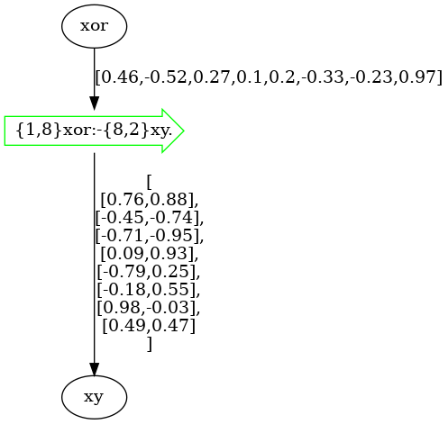
All that is needed to visualize the model - the template with current weights’ values is to call the draw method.
from neuralogic.utils.data import XOR_Vectorized


template, dataset = XOR_Vectorized()
model = template.build()

model.draw()
Tip
You can also visualize the template by calling the template.draw method.
Templates (models) and samples can be drawn into various raster formats (such as PNG or JPEG) or SVG format, which is
considerably faster for larger graphs. To set the format, simply use the img_type parameter.
The drawing can be further parameterized, for example, with the value_detail parameter to display more (or less) decimal
places of all values (there are three levels of detail - 0-2, where 0 has the least number of decimals
and 2 the most number of decimals).
The model above was directly drawn into Jupyter Notebook without any parametrization.
To draw the model into a file, all we have to do is add the filename parameter with a path to the output image, such as:
model.draw(filename="my_image.png")
We can also get raw images bytes by turning off displaying into IPython:
model.draw(show=False)
Samples Rendering
Samples can be drawn in the same way and supports the same parametrization as the model drawing.
An example of drawing samples can be seen in the code below, where we render the actual computation graph for the first example (input [0, 0]).
built_dataset = model.build_dataset(dataset)

built_dataset.samples[0].draw()
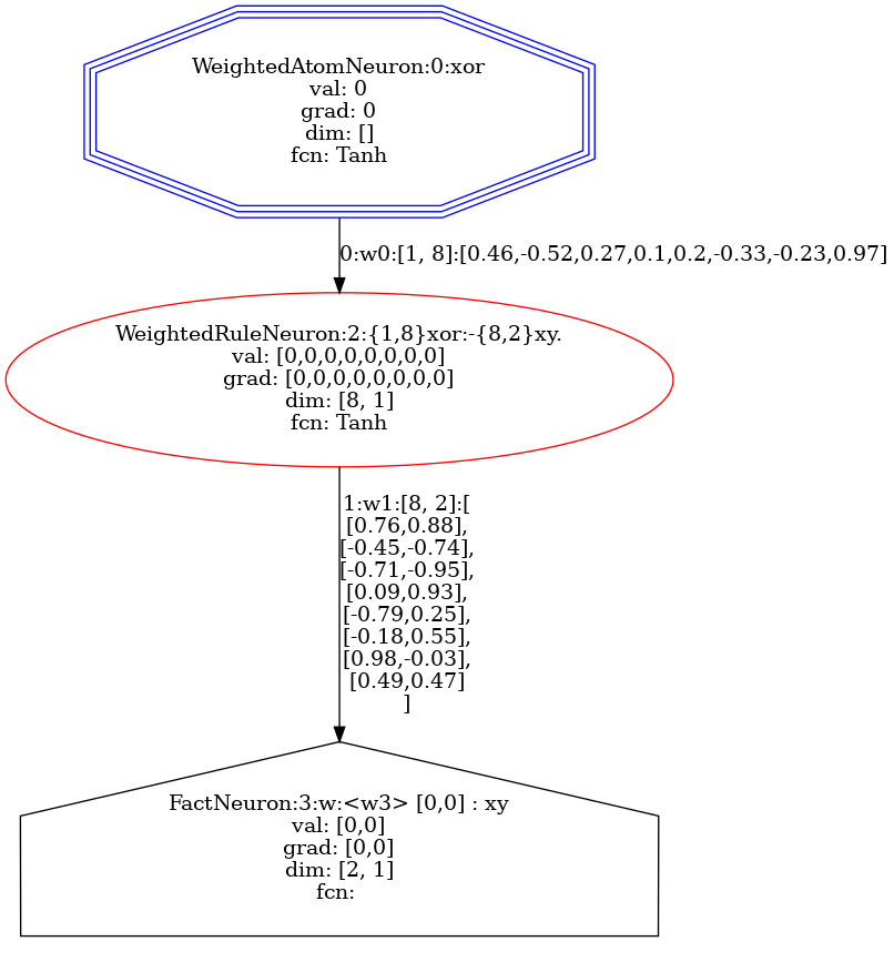
Getting the DOT Source
To get the DOT source of the model or the sample, all you have to do is call the model_to_dot_source function or
the sample_to_dot_source function, respectively.
from neuralogic.utils.visualize import sample_to_dot_source


dot_source = sample_to_dot_source(built_dataset.samples[0])
print(dot_source)
digraph G {
3 [shape=house, color=black, label="FactNeuron:3:w:<w3> [0,0] : xy
val: [0,0]
grad: [0,0]
dim: [2, 1]
fcn:
"]

2 [shape=ellipse, color=red, label="WeightedRuleNeuron:2:{1,8}xor:-{8,2}xy.
val: [0,0,0,0,0,0,0,0]
grad: [0,0,0,0,0,0,0,0]
dim: [8, 1]
fcn: Tanh
"]
2 -> 3 [label="1:w1:[8, 2]:[
[0.76,0.88],
[-0.45,-0.74],
[-0.71,-0.95],
[0.09,0.93],
[-0.79,0.25],
[-0.18,0.55],
[0.98,-0.03],
[0.49,0.47]
]"]

0 [shape=ellipse, color=blue, label="WeightedAtomNeuron:0:xor
val: 0
grad: 0
dim: []
fcn: Tanh
"]
0 -> 2 [label="0:w0:[1, 8]:[0.46,-0.52,0.27,0.1,0.2,-0.33,-0.23,0.97]"]

0 [shape = tripleoctagon]
}